In this project, we explore the usage of diffusion models for the purposes of image generation
and editing.
Part A: The Power of Diffusion Models!
As the first part of the project, we use the existing, pretrained DeepFloyd IF diffusion model
and precomputed text embeddings to creating sampling loops and perform image editing tasks.
Part 1: Sampling Loops
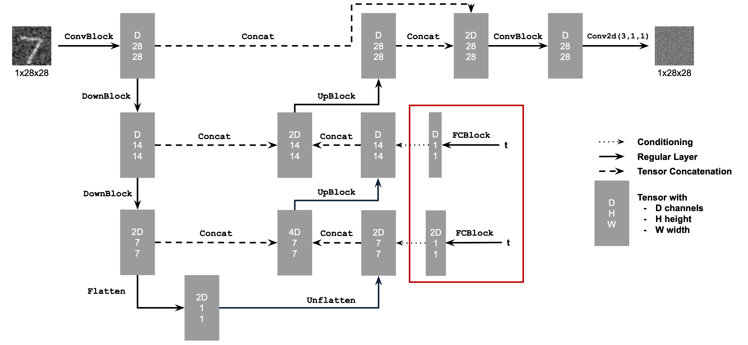
The main idea between our diffusion models is to train a neural net that can iteratively reverse
the noising process of an image. This way, we have a model that incremental takes a noisy image
and moves it towards the desired image manifold, allowing us to generate new images.
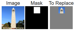
1.1: Implementing the Forward Process
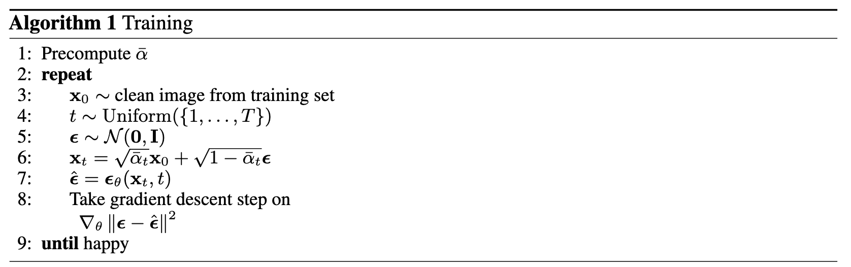
In order to do this, we first need to be able to add noise to images at our desired threshold.
The equation that achieves this is:
$$x_t = \sqrt{\bar{\alpha_t}}x_0 + \sqrt{1 - \bar{\alpha_t}}\epsilon$$
where \(\epsilon \sim N(0,1)\) is sampled at random. This is implemented in
forward(im, t).
Our \(\bar{\alpha_t}\) variable is taken from the array
alphas_cumprod, which gives
us magnitudes for the desired noise at the different time periods. Below are the results of applying
this forward method on an image of the Campanile for \(t \in [250, 500, 750]\):
 Image of the Campanile.
|
 Noised at t=250.
|
 Noised at t=500.
|
 Noised at t=750.
|
1.2: Classical Denoising
Before we use our pretrained neural nets to denoise the image, we first demonstrate the results
of classical noising techniques via a low pass filter. Below are the results for the previously
noised images:
|
Noised at t=250.
|
Noised at t=500.
|
Noised at t=750.
|
 Gaussian blur denoise at t=250.
|
Gaussian blur denoise at t=500.
|
Gaussian blur denoise at t=750.
|
As we can see, this method isn't very effective especially at high noise levels. Note a kernel size of 15
and a \sigma of 2 were used in the gaussian blurs.
1.3: One-Step Denoising
Now we can actually try using our neural net to denoise the image. For now, we will try and
estimate the original image in one step. Our neural net gives us a noise estimate \(\epsilon\) given the
noised image and the timestep t, and we can then recover the estimated original image by
solving for \(x_0\) in the original forward pass, giving:
$$x_0 = \frac{x_t - \sqrt{1 - \bar{\alpha_t}}\epsilon}{\sqrt{\bar{\alpha_t}}}$$
Applying this formula, we get the following results:
|
Noised at t=250.
|
Noised at t=500.
|
Noised at t=750.
|
 One-step denoise at t=250.
|
One-step denoise at t=500.
|
One-step denoise at t=750.
|
As we can see, this results are much better than those obtained using classical denoising in
part 1.2.
1.4: Iterative Denoising
We can further improve this denoising process by iteratively denoising the image, instead of
simply trying to do it in one pass. This can be thought of as each step taking a linear interpolated
step for our current state towards the estimated clean image produced by 1.3. Additionally, instead
of strictly iterating step by step down the values of t, we can take strided steps. For these examples,
we will take strided steps of 30 from 990 to 0. The iterative step is defined below:
$$x_{t'} = \frac{\sqrt{\bar{\alpha_{t'}}}\beta_t}{1 - \bar{\alpha_t}}x_0 + \frac{\sqrt{\alpha_t}(1-\bar{\alpha_{t'}})}{1-\bar{\alpha_t}}x_t + v_\sigma$$
where \(x_t\) is our current image, \(x_0\) is the estimate of the original image detailed in
part 1.3, \(\bar{\alpha_t}\) is as defined before from
alphas_cumprod, \(\alpha_t = \frac{\bar\alpha_t}{\bar\alpha_{t'}}\),
\(\beta_t = 1 - \alpha_t\), and \(v_\sigma\) is a predicted noise that is also outputted by DeepFloyd.
Then, with
t_start = 10, iterating following these steps along our
strided_timesteps gives us the following results
(with comparison to our methods provided):
 Denoised at t=90.
|
 Denoised at t=240.
|
 Denoised at t=390.
|
 Denoised at t=540.
|
 Denoised at t=690.
|
|
Original.
|
 Iteratively denoised.
|
 One-step denoise.
|
 Gaussian blurred denoise.
|
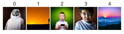
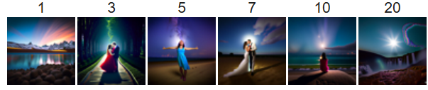
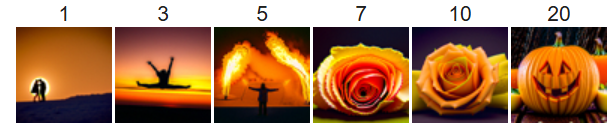
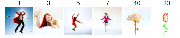
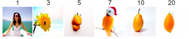
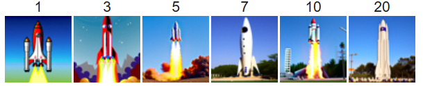
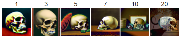
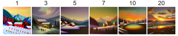
1.5: Diffusion Model Sampling
We can actually use our
iterative_denoise function from part 1.4 to also generate
new images. This is done by setting
t_start = 0 and passing in random noise as our
images. Five sampled images are shown below using this method:
 5 sampled images using iterative denoising.
|